The Dias (2000) model

Introduction

The model proposed by Dias (1972) describes the petrophysical properties of rocks from measurements of their electrical polarization in a frequency range typically from 1 mHz to 100 kHz.

We refer to Dias (2000) for the implementation of the complex resistivity formula in BISIP. This model predicts that the complex resistivity spectra \(\rho^*\) of a polarizable rock sample can be described by

\begin{equation} \rho^* = \rho_0 \left[ 1-m\left(1-\frac{1}{1+i\omega\tau'\left(1+\frac{1}{\mu}\right)} \right) \right], \end{equation}

where \(\omega\) is the measurement angular frequencies (\(\omega=2\pi f\)) and \(i\) is the imaginary unit. Additionally,

\begin{equation} \mu = i\omega\tau + \left(i\omega\tau''\right)^{1/2}, \end{equation}

\begin{equation} \tau' = (\tau/\delta)(1 - \delta)/(1 - m), \end{equation}

\begin{equation} \tau'' = \tau^2 \eta^2. \end{equation}

Here, \(\rho^*\) depends on 5 parameters:

• \(\rho_0 \in [0, \infty)\), the direct current resistivity \(\rho_0 = \rho^*(\omega\to 0)\).
• \(m \in [0, 1)\), the chargeability \(m=(\rho_0 - \rho_\infty)/\rho_0\).
• \(\tau \in [0, \infty)\), the relaxation time, related to average polarizable particle size.
• \(\eta \in [0, 150]\), characteristic of the electrochemical environment producing polarization.
• \(\delta \in [0, 1)\), the pore length fraction of the electrical double layer zone in the material.

In this tutorial we will invert a SIP data with the Dias model to explore the parameter space of this semi-empirical SIP model. We will also quantify the relationship between the various parameters.

Exploring the parameter space

First import the required packages.

import os

import numpy as np
from IPython.display import display, Math
from bisip import Dias2000
from bisip import DataFiles

np.random.seed(42)

To invert a SIP data file with the Dias model, start by instantiating a Dias2000 object and call the fit() method to estimate the parameters.

# This will get one of the example data files in the BISIP package
data_files = DataFiles()
filepath = data_files['SIP-K389172']

# Define MCMC parameters and Dias model
nwalkers = 32
nsteps = 1000
model = Dias2000(filepath=filepath, nwalkers=nwalkers, nsteps=nsteps)
# Fit model to data
model.fit()

100%|██████████| 1000/1000 [00:01<00:00, 511.36it/s]

fig = model.plot_traces()

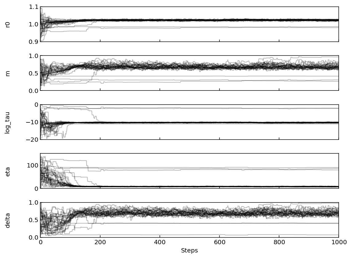
Some walkers get stuck in local minima because the priors are really wide. Nevertheless, we can see that the median solution of all these chains gives a satisfying result.

# Plot the fit by discarding the first 500 steps
fig = model.plot_fit(discard=500)

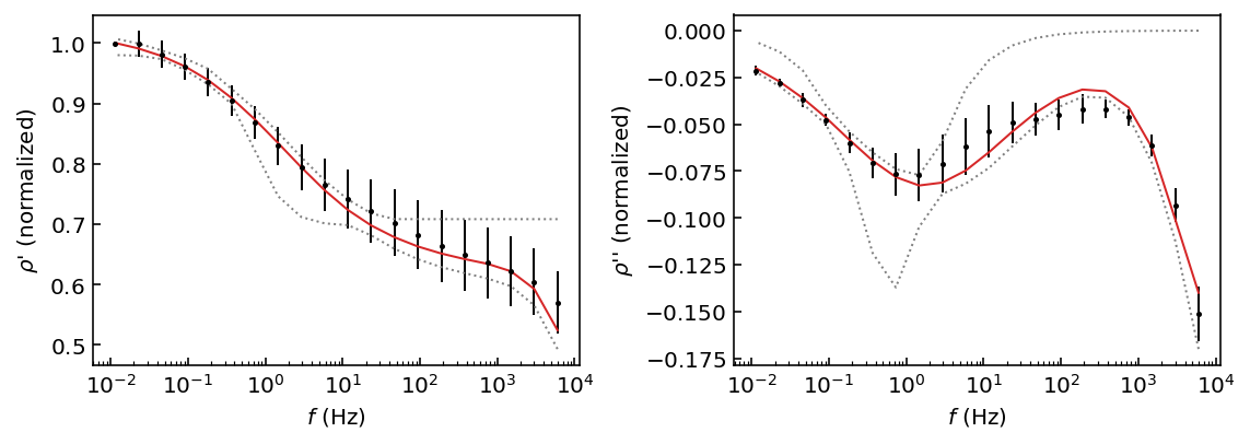
The adjustment is satisfying, but the 95% HPD is very wide because some of the walkers were stuck in local minima far from the solution. A good strategy to reduce the chance that walkers get stuck in local minima would be to tighten the priors are the values we think give a good result. Here we will set new boundaries for \(\eta\) and \(\log \tau\).

# Adjust the boundaries
model.params.update(eta=[0, 25], log_tau=[-15, -5])

model.fit()
fig = model.plot_traces()

100%|██████████| 1000/1000 [00:01<00:00, 533.24it/s]

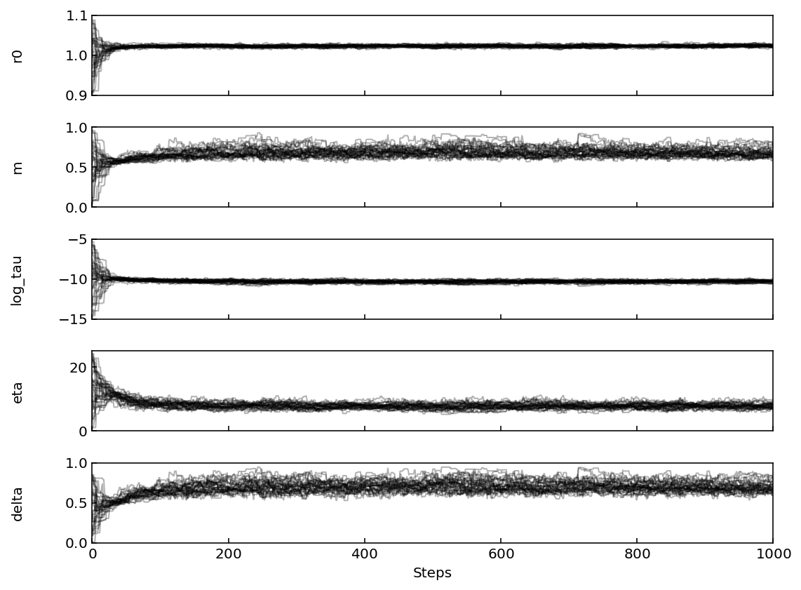
The stricter priors have allowed all walkers to find a similar stationary state. With these improved parameter chains the fit quality should be improved.

# Plot the fit by discarding the first 500 steps
fig = model.plot_fit(discard=500)

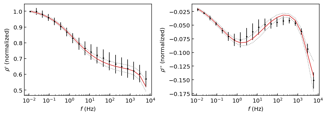
The adjustment is satisfying, and the 95% HPD reasonable if we consider the measurement error bars. We will now visualize the posterior distribution of the Dias model with the plot_corner method.

# Plot the posterior by discarding the first 500 steps
fig = model.plot_corner(discard=500)

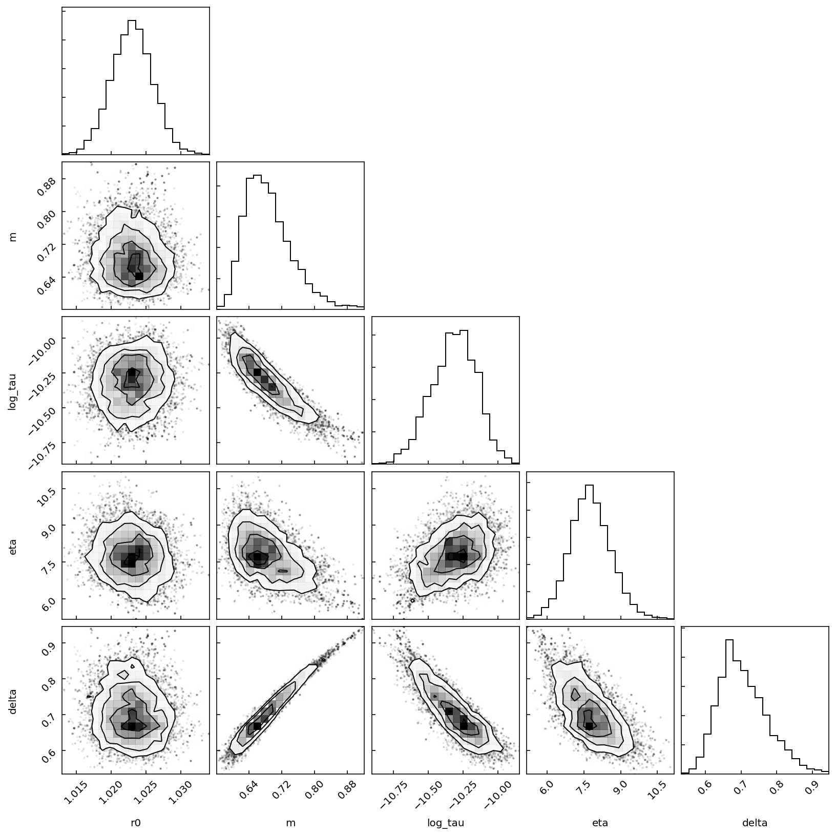
The corner plot shows interesting correlations between various parameters. Finally, let’s look at the optimal parameters and their uncertainties.

# Use this utility function to nicely print parameter values
# for the Dias model with LaTeX

# Print the mean and std of the parameters after discarding burn-in samples
values = model.get_param_mean(discard=500)
uncertainties = model.get_param_std(discard=500)

model.print_latex_parameters(model.param_names, values, uncertainties)

$\displaystyle \rho_0: 1.023 \pm 0.003$

$\displaystyle m: 0.688 \pm 0.058$

$\displaystyle \log\tau: -10.315 \pm 0.162$

$\displaystyle \eta: 7.767 \pm 0.838$

$\displaystyle \delta: 0.707 \pm 0.068$

Conclusions

From this experiment, we conclude that the \(\rho_0\) parameter is relatively independent from the others. We also note that \(m\) and \(\tau\) are characterized by a strong correlation coefficient. Most importantly, we find that this correlation makes the range of ‘best’ values for these parameters quite large, indicating that these parameters are not well resolved for this particular data file.